Though BI Tools are available with the MS Dynamics Ax
2012, and Third Party Tools for creating BI Reports and Models are available in
the market. But emergence of Power Query, Power View, Power Pivot, and Power
BI, with MS Excel turned the BI development to a new horizon.
As it is known that Microsoft Dynamics AX 2012 provides
a flexible pre-built business intelligence (BI) solution for mid-market
organizations. The use of built-in content—including Role Centers, analytic
reports, and analysis cubes—eliminates the need to build a solution from the
ground up, and therefore saves time and money. The Microsoft Dynamics AX 2012
business intelligence solution can be configured and extended to suit your
specific needs with the help of Microsoft Business Intelligence development
tools.
The Microsoft Dynamics AX 2012 business intelligence
solution consists of the following built-in features:
1.
Role Centers (dashboards):
Thirty-two default home pages that pertain to the work needs of various user
profiles in an organization.
2.
Analysis cubes: Eleven analysis cubes
that address the analytic requirements of the major functional areas within
Microsoft Dynamics AX 2012—including finance, supply chain, manufacturing,
professional services, and business processes.
3.
Key Performance Indicators (KPIs):
More than 60 of the most commonly used KPIs that help users evaluate the
success of business activities.
4.
Analytic reports: More than 150 analytic
reports that provide insight into business data.
No doubt these are sufficient enough for the user. But
development or modification needs customer support (development team). Further,
integration services, again requires a customer support.
Power Query is a free Add-in to Excel add-in that can be
used for data discovery, reshaping the data and combining data coming from
different sources. Power Query is one of the Excel add-ins provided as part of
Microsoft Power BI self-service solution.
This is an ETL tool (Extract, Transform, Load – like SSIS)
built into your familiar Excel to search or discover data from a wide variety
of data sources (both from your enterprise as well as from online public data
sources). Power Query has an intuitive and interactive user interface which can
be used to search, discover, acquire, combine, refine, transform and enrich the
data.
Power Pivot is a free add-in to Excel, it extends the
capabilities of the pivot table data summarization and cross-tabulation feature
with new features such as expanded data capacity, advanced calculations,
ability to import data from multiple sources, and the ability to publish the
workbooks as interactive web applications. As such, Power Pivot falls under
Microsoft's Business Intelligence offering, complementing it with its
self-service, in-memory capabilities.
Let us make some analytical reports by using the Power
Tools of Microsoft.
In this walk through we will design two refreshable
(updatable) reports with the help of the Microsoft’s Power Tools.
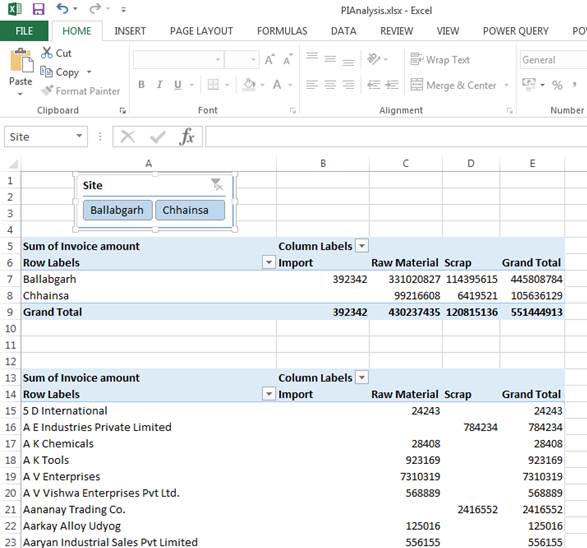
The first picture depicts analysis of Invoice Amounts of
Purchases of two sites, one is Ballabgarh and another is Chhainsa. Also there
are three types of Purchases eg Raw Material, Scrap and Import (these types are
indigenous or local to the organisation).

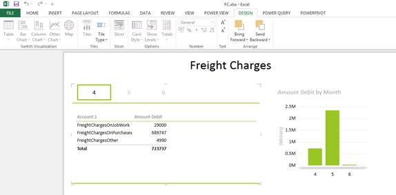
The second picture shows analysis of one expense account
named Freight Charges with different dimensions for different months, this data
is being transferred from a SSRS Report.

Make the First Report:
1.
Select
menu option Invoice Journal from the Inquiries Menu group from Accounts Payable
module, as shown below.

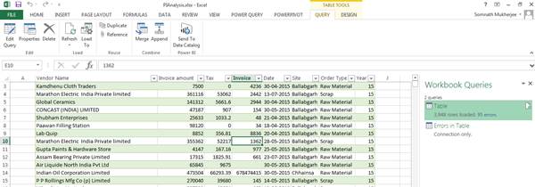
2.
A
list of transaction will appear in the form of grid form. It will show a list
of Invoice Account, Purchase Order, Date, Invoice, Voucher, Tax, Invoice Amount
etc.
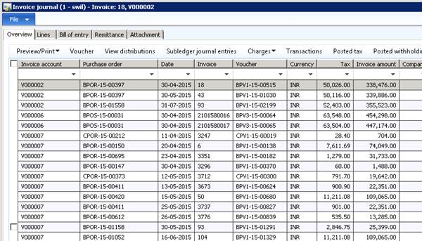
3.
Press
Ctrl+T to export the grid data to an excel file.
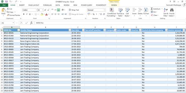
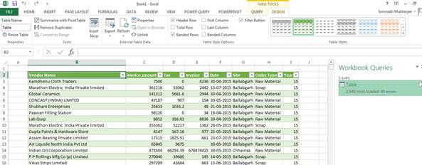
This data in excel is in the form of Table (Excel Table),
with all the properties of Excel Table, like Automatic Filterable, Sortable,
able to Pivot etc. Save the table with a Name, say e.g. PurchaseInvoice.xlsx.
4.
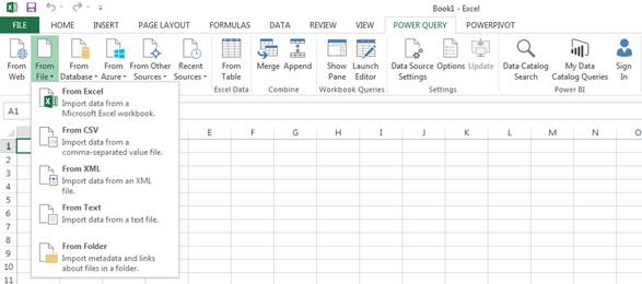
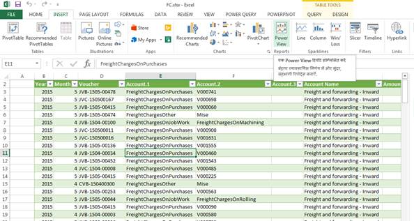
Now
open a new Excel File. Select option From File from Menu Group Get
External Data of the Power Query Tab. If you do not have Power Query
Add-ins, please install the power query (it is a free tool from Microsoft).
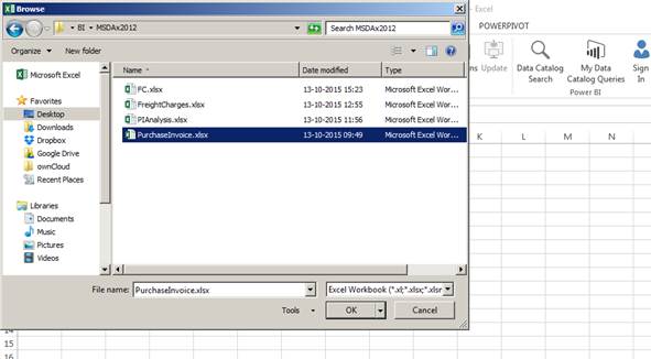
Select the Form Excel menu option.
Select the File with the help of the File Dialog Box.
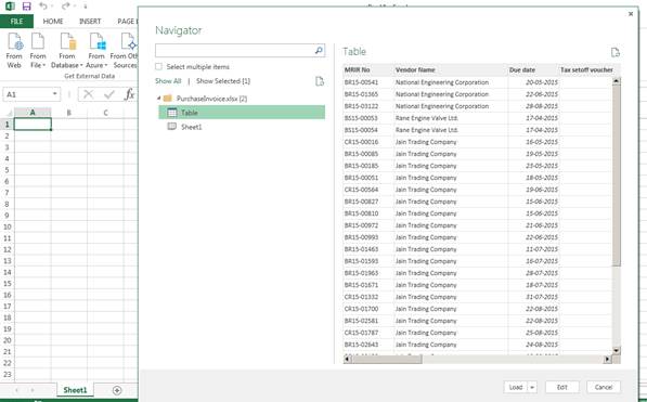
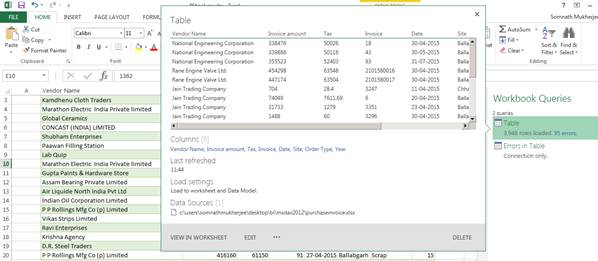
After selecting the Excel File, the following Navigator
will appear. Select the Table and not the sheet, as you have exported the data
in the form of Table having a Table Name.
5.
Click
Edit Button, as we want to transform the data, after Extraction.
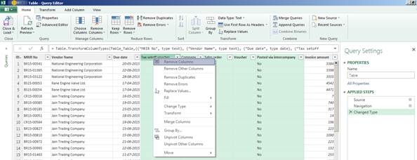
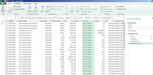
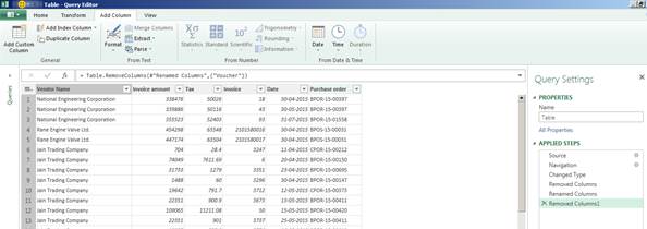
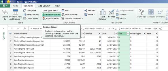
Please note that each
activity done here is being recorded as a query command. To remove any
un-wanted column, select the columns and then remove it by using button from
the Manage Columns group or context menu could be used.
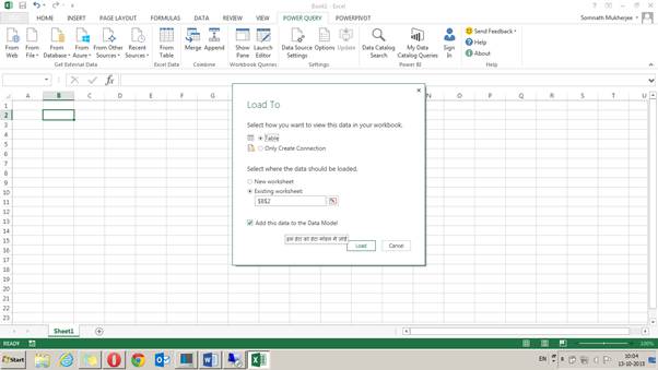
6.
Click
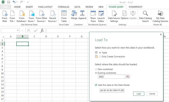
the Close & Load button from the Close
Menu Group. This will ask if you want to load the data as a table or want to
record this as a connection (to be used later on after some more extraction and
transformation).
After loading the query could be edited by opening the
workbook query from the option shown right to the excel table. Also all the
data could be refreshed with new or modified data. One has to export the excel
data from MS Dynamics to Excel Table and replacing the file
PurchaseInvoice.Xlsx in this case.
As you have seen that the ETL commands are recorded in
the workbook itself, any command can be deleted or added or modified after its
creation.

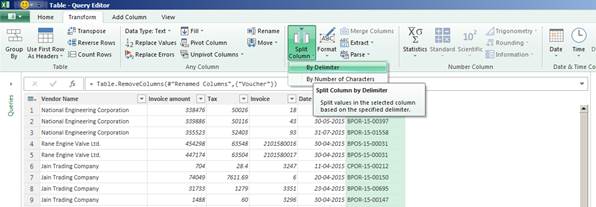
7.
Now,
let us split one of the column, Purchase Order.
Splitting can be done in
two ways, by some delimiter or some number of characters. Here let us use the
option by Delimiter.
8.
Select
the Column Purchase Order and Select the menu option By Delimiter.
This will ask for some parameters like Delimiter type,
here sign (-) is a custom type of delimiter. Then put the (-) in the second
text box and then select the split radio button (At each occurrence),
and click ok.
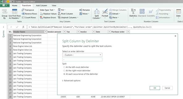
This will split the Purchase Order into three columns as
show below.
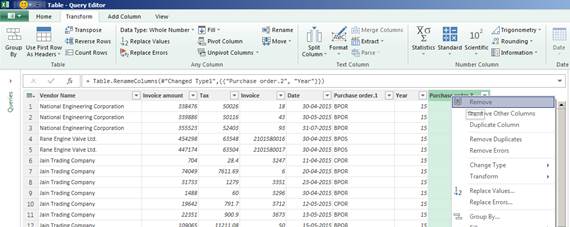
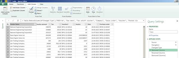
Now remove some un-wanted columns. Not to repeat that
these queries are being recorded into the workbook, for reprocessing
automatically during later use. So repetition of ETL is not need.
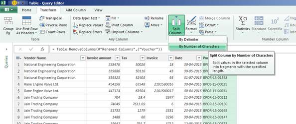
9.
Let
us use the split function by character. Here we need B/C from the first
character of the Purchase Order first chunk, also we need R/I/S from the Fourth
character of the first chunk like BPOR (we need B and R). So, select the Split
Columns-> By Number of Characters after selecting the Column showing
BPOR (that is Purchase order.1 column). Provide the parameter as required, shown
below.
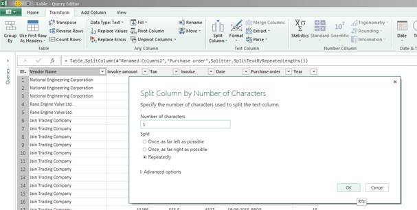
This will split each character by one column, as shown
below. Rename the columns.
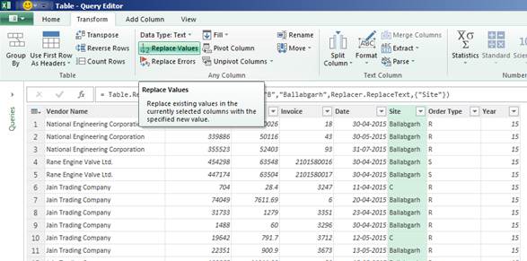
10.
Now
let us use the replace tool, in the Site Column, replace all B with Ballabgarh,
and C with Chhainsa.
In the same way replace in the Order Type Column, R with
Raw Material, S with Scrap, I with Import, as shown below.
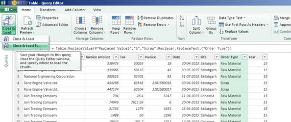
11.
Now
Close & Load the Data.
Following set of data would load. As you can see it is
showing some errors (95 errors), by clicking the hyperlink one can view the
errors.
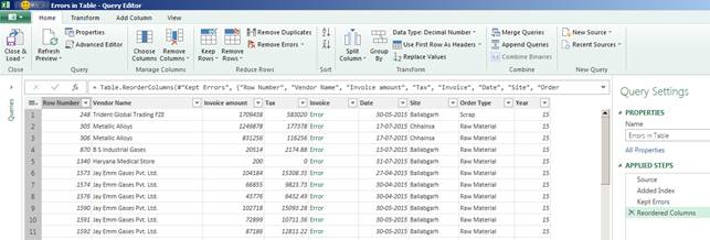
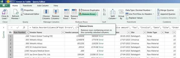
These Errors could be removed by using several ETL
techniques. In this example we could use the Remove Errors button
from the Reduce Rows menu group.
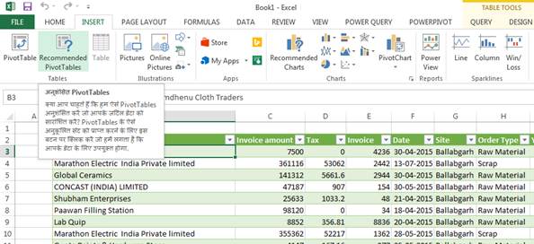
12.
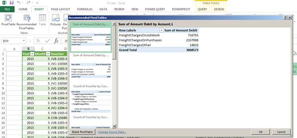
Now
one can use some of the Excel’s new feature available in 2013 version, like
recommended Pivot Tables and Pivot Charts. Here is an example
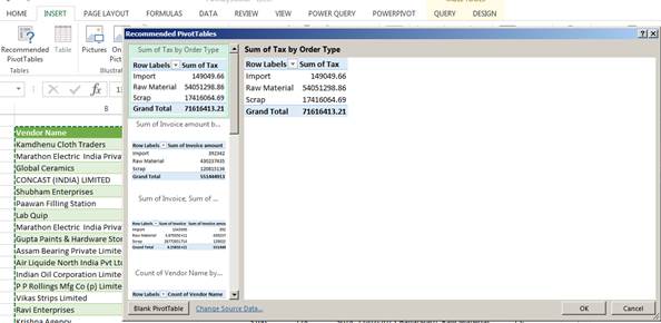
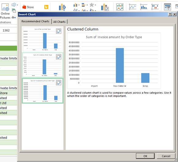
By using a Pivot Table, Slicer, and Pivot Chart, some
analysis of the data is shown below.
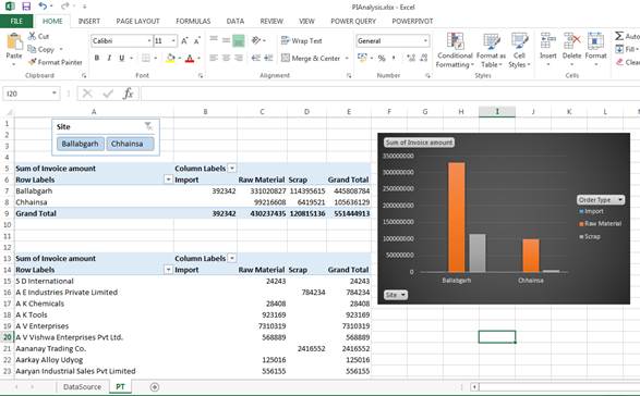
This data could be refreshed or modified any time when
required.
Make the Second Report:
1.
Selected
a customized report from the Report menu group.
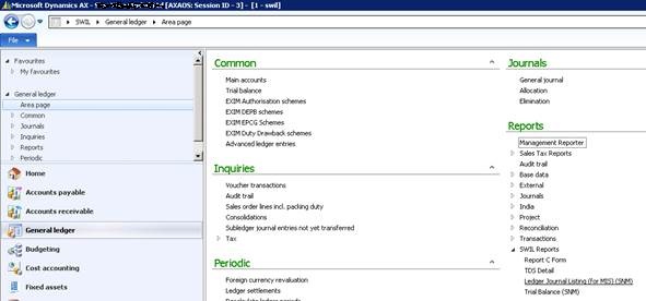
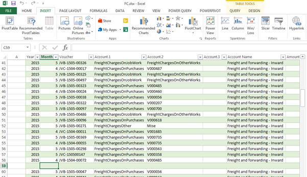
The report looks like as shown below.
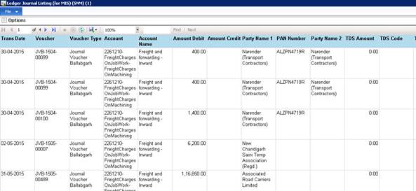
Save this report with as Excel with a name FreightCharges.xlsx
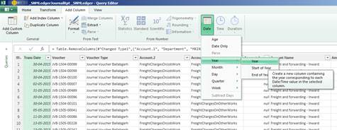
2.
Transform
the Column Date to get Year and Month from the date type of data. This will add
two columns Year and Month.
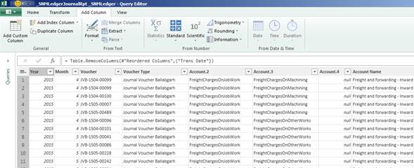
3.
After
all Transformation the data will look like as shown below.
4.
To
remove any null row use filter query by using the drop-down in the ETL form.
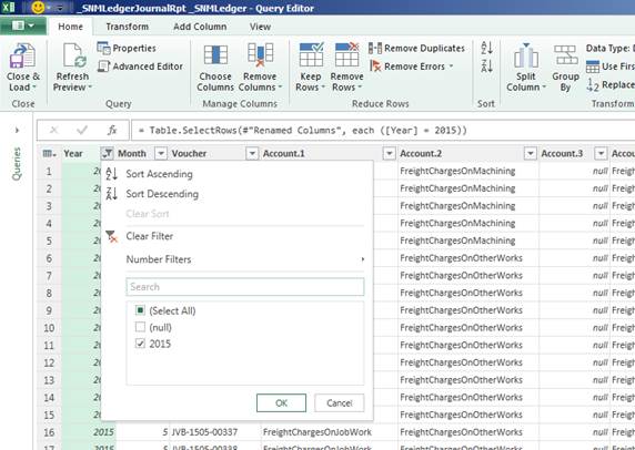
This will generate a filtering query in the workbook.
Then create Pivot Table as it was done in the First Example.
5.
To
make use of Power View click on the Power View Button in the
Report Group, as shown below.
To have a knowledge of Power View, Power Query, Power
Pivot, Power BI, please visit websites and blogs.